Statistics: Elementary Probability Theory

Elementary Probability Theory

Statistics: Elementary Probability Theory

A probability gives the likelihood that a defined event will occur. It is quantified as a positive number between 0 (the event is impossible) and 1 (the event is certain). Thus, the higher the probability of a given event, the more likely it is to occur. If A is a defined event, then the probability of A occurring is expressed as P(A). Probability can be expressed in a number of ways. A frequentist approach is to observe a number of particular events out of a total number of events. Thus, we might say the probability of a boy is 0.52, because out of a large number of singleton births we observe 52% are boys. A model based approach is where a model, or mechanism determines the event; thus, the probability of a ‘1’ from an unbiased die is 1/6 since there are 6 possibilities, each equally likely and all adding to one. An opinion based approach is where we use our past experience to predict a future event, so we might give the probability of our favourite football team winning the next match, or whether it will rain tomorrow.

Given two events A and B, we often want to determine the probability of either event, or both events, occurring.

Addition Rule

The addition rule is used to determine the probability of at least one of two (or more) events occurring. In general, the probability of either event A or B is given by:

P(A or B) = P(A) + P(B) – P(A and B)

If A and B are mutually exclusive, this means they cannot occur together, i.e. P(A and B)=0. Therefore, for mutually exclusive events the probability of either A or B occurring is given by:

P(A or B) = P(A) + P(B)

Example: If event A is that a person is blood group O and event B is that they are blood group B, then these events are mutually exclusive since a person may only be either one or the other. Hence, the probability that a given person is either group O or B is P(A)+P(B).

Multiplication Rule

The multiplication rule gives the probability that two (or more) events happen together. In general, the probability of both events A and B occurring is given by:

P(A and B) = P(A) x P(B|A) = P(B) x P(A|B)

The notation P(B|A) is the probability that event B occurs given that event A has occurred where the symbol ‘|’ is read is ‘given’. This is an example of a conditional probability, the condition being that event A has happened. For example, the probability of drawing the ace of hearts from a well shuffled pack is 1/51. The probability of the ace of hearts given that the card is red is 1/26.

Example: If event A is a person getting neuropathy and event B that they are diabetic, then P(A|B) is the probability of getting neuropathy given that they are diabetic.

If A and B are independent events, then the probability of event B is unaffected by the probability of event A (and vice versa). In other words, P(B|A) = P(B). Therefore, for independent events, the probability of both events A and B occurring is given by:

P(A and B) = P(A) x P(B)

Example: If event A is that a person is blood group O and event B that they are diabetic, then the probability of someone having blood group O and being diabetic is P(A)xP(B), assuming that getting diabetes is unrelated to a person’s blood group.

Note that if A and B are mutually exclusive, then P(A|B)=0

Bayes’ Theorem

From the multiplication rule above, we see that:

P(A) x P(B|A) = P(B) x P(A|B)

This leads to what is known as Bayes' theorem:

$P (B | A) = \frac{P (A | B) P (B)}{P (A)}$

Thus, the probability of B given A is the probability of A given B, times the probability of B divided by the probability of A.

This formula is not appropriate if P(A)=0, that is if A is an event which cannot happen.

An example of the use of Bayes’ theorem is given below.

Sensitivity and Specificity

Many diagnostic test results are given in the form of a continuous variable (that is one that can take any value within a given range), such as diastolic blood pressure or haemoglobin level. However, for ease of discussion we will first assume that these have been divided into positive or negative results. For example, a positive diagnostic result of 'hypertension' is a diastolic blood pressure greater than 90 mmHg; whereas for 'anaemia', a haemoglobin level less than 12 g/dl is required.

For every diagnostic procedure (which may involve a laboratory test of a sample taken) there is a set of fundamental questions that should be asked. Firstly, if the disease is present, what is the probability that the test result will be positive? This leads to the notion of the sensitivity of the test. Secondly, if the disease is absent, what is the probability that the test result will be negative? This question refers to the specificity of the test. These questions can be answered only if it is known what the 'true' diagnosis is. In the case of organic disease this can be determined by biopsy or, for example, an expensive and risky procedure such as angiography for heart disease. In other situations it may be by 'expert' opinion. Such tests provide the so-called 'gold standard'.

Example

Consider the results of an assay of N-terminal pro-brain natriuretic peptide (NT-proBNP) for the diagnosis of heart failure in a general population survey in those over 45 years of age, and in patients with an existing diagnosis of heart failure, obtained by Hobbs, Davis, Roalfe, et al (BMJ 2002) and summarised in table 1. Heart failure was identified when NT-proBNP > 36 pmol/l.

Table 1: Results of NT-proBNP assay in the general population over 45 and those with a previous diagnosis of heart failure (after Hobbs, David, Roalfe et al, BMJ 2002)

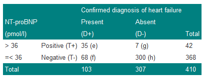
We denote a positive test result by T+, and a positive diagnosis of heart failure (the disease) by D+. The prevalence of heart failure in these subjects is 103/410=0.251, or approximately 25%. Thus, the probability of a subject chosen at random from the combined group having the disease is estimated to be 0.251. We can write this as P(D+)=0.251.

The sensitivity of a test is the proportion of those with the disease who also have a positive test result. Thus the sensitivity is given by e/(e+f)=35/103=0.340 or 34%. Now sensitivity is the probability of a positive test result (event T+) given that the disease is present (event D+) and can be written as P(T+|D+), where the '|' is read as 'given'.

The specificity of the test is the proportion of those without disease who give a negative test result. Thus the specificity is h/(g+h)=300/307=0.977 or 98%. Now specificity is the probability of a negative test result (event T-) given that the disease is absent (event D-) and can be written as P(T-|D-).

Since sensitivity is conditional on the disease being present, and specificity on the disease being absent, in theory, they are unaffected by disease prevalence. For example, if we doubled the number of subjects with true heart failure from 103 to 206 in Table 1, so that the prevalence was now 103/(410+103)=20%, then we could expect twice as many subjects to give a positive test result. Thus 2x35=70 would have a positive result. In this case the sensitivity would be 70/206=0.34, which is unchanged from the previous value. A similar result is obtained for specificity.

Sensitivity and specificity are useful statistics because they will yield consistent results for the diagnostic test in a variety of patient groups with different disease prevalences. This is an important point; sensitivity and specificity are characteristics of the test, not the population to which the test is applied. In practice, however, if the disease is very rare, the accuracy with which one can estimate the sensitivity may be limited. This is because the numbers of subjects with the disease may be small, and in this case the proportion correctly diagnosed will have considerable uncertainty attached to it.

Two other terms in common use are: the false negative rate (or probability of a false negative) which is given by f/(e+f)=1-sensitivity, and the false positive rate (or probability of a false positive) or g/(g+h)=1-specificity.

These concepts are summarised in Table 2.

Table 2: Summary of definitions of sensitivity and specificity

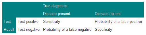
It is important for consistency always to put true diagnosis on the top, and test result down the side. Since sensitivity=1–P(false negative) and specificity=1–P(false positive), a possibly useful mnemonic to recall this is that 'sensitivity' and 'negative' have 'n's in them and 'specificity' and 'positive' have 'p's in them.

Predictive Value of a Test

Suppose a doctor is confronted by a patient with chest pain suggestive of angina, and that the results of the study described in Table 3 are available.

Table 3: Results of exercise tolerance test in patients with suspected coronary artery disease

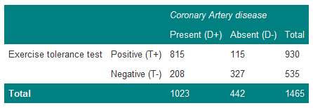
The prevalence of coronary artery disease in these patients is 1023/1465=0.70. The doctor therefore believes that the patient has coronary artery disease with probability 0.70. In terms of betting, one would be willing to lay odds of about 7:3 that the patient does have coronary artery disease. The patient now takes the exercise test and the result is positive. How does this modify the odds? It is first necessary to calculate the probability of the patient having the disease, given a positive test result. From Table 3, there are 930 men with a positive test, of whom 815 have coronary artery disease. Thus, the estimate of 0.70 for the patient is adjusted upwards to the probability of disease, with a positive test result, of 815/930=0.88.

This gives the predictive value of a positive test (positive predictive value):

P(D+|T+) = 0.88.

The predictive value of a negative test (negative predictive value) is:

P(D-|T-) = 327/535 = 0.61.

These values are affected by the prevalence of the disease. For example, if those with the disease doubled in Table 3, then the predictive value of a positive test would then become 1630/(1630+115)=0.93 and the predictive value of a negative test 327/(327+416)=0.44.

The Role of Bayes' Theorem

Suppose event A occurs when the exercise test is positive and event B occurs when angiography is positive. The probability of having both a positive exercise test and coronary artery disease is thus P(T+ and D+). From Table 3, the probability of picking out one man with both a positive exercise test and coronary heart disease from the group of 1465 men is 815/1465=0.56.

However, from the multiplication rule:

P(T+ and D+) = P(T+|D+)P(D+)

P(T+|D+)=0.80 is the sensitivity of the test and P(D+)=0.70 is the prevalence of coronary disease and so P(T+ and D+)=0.80x0.70=0.56, as before.

Bayes' theorem enables the predictive value of a positive test to be related to the sensitivity of the test, and the predictive value of a negative test to be related to the specificity of the test. Bayes' theorem enables prior assessments about the chances of a diagnosis to be combined with the eventual test results to obtain a so-called “posterior” assessment about the diagnosis. It reflects the procedure of making a clinical judgement.

In terms of Bayes' theorem, the diagnostic process is summarised by:

$P (D + | T +) = \frac{P (T + | D +) P (D +)}{P (T +)}$

The probability P(D+) is the a priori probability and P(D+|T+) is the a posteriori probability.

Bayes' theorem is usefully summarised when we express it in terms of the odds of an event, rather than the probability. Formally, if the probability of an event is p, then the odds are defined as p/(1-p). The probability that an individual has coronary heart disease, before testing, from the Table is 0.70, and so the odds are 0.70/(1-0.70)=2.33 (which can also be written as 2.33:1).

Likelihood Ratio

In terms of odds we can summarise Bayes' theorem using what is known as the positive likelihood ratio (LR+), defined as:

$L R + = \frac{P (T + | D +)}{P (T + | D -)} = \frac{S e n s i t i v i t y}{1 - S p e c i f i c i t y}$

Thus the Likelihood Ratio of a positive test is the probability of getting a positive result when a subject has the disease, to the probability of a positive test given the subject does not have the disease.

It can be shown that Bayes' theorem can be summarised by:

Odds of disease after test = Odds of disease before test x likelihood ratio

From Table 3, the likelihood ratio is 0.80/(1–0.74)=3.08, and so the odds of the disease after the test are 3.08x2.33=7.2. This can be verified from the post-test probability of 0.88 calculated earlier, so that the post-test odds are 0.88/(1–0.88)=7.3. (This differs from the 7.2 because of rounding errors in the calculation.)

Example

This example illustrates Bayes' theorem in practice by calculating the positive predictive value for the data of Table 3.

We use the formula

$P (D + | T +) = \frac{P (T + | D +) P (D +)}{P (T +)}$

From the Table: P(T+)=930/1465=0.63, P(D+)=0.70 and P(T+|D+)=0.80, thus:

Positive predictive value = (0.8 x 0.7)/0.63 = 0.89

.…which is what we previously calculated (bar a small rounding error).

Example

The prevalence of a disease is 1 in 1000, and there is a test that can detect it with a sensitivity of 100% and specificity of 95%. What is the probability that a person has the disease, given a positive result on the test?

Many people, without thinking, might guess the answer to be 0.95, the specificity.

Using Bayes' theorem, however:

$P (D + | T +) = \frac{S e n s i t i v i t y \times P r e v a l e n c e}{P r o b a b i l i t y o f p o s i t i v e r e s u l t}$

To calculate the probability of a positive result, consider 1000 people in which one person has the disease. The test will certainly detect this one person. However, it will also give a positive result on 5% of the 999 people without the disease. Thus, the total positives is 1+(0.05x999)=50.95 and the probability of a positive result is 50.95/1000=0.05095.

Thus:

$P (D + | T +) = \frac{1 \times 0.001}{0.05095} = 0.02$

The usefulness of a test will depend upon the prevalence of the disease in the population to which it has been applied. In general, a useful test is one which considerably modifies the pre-test probability. If the disease is very rare or very common, then the probabilities of disease given a negative or positive test are relatively close and so the test is of questionable value.

Independence and Mutually Exclusive Events

In Table 3, if the results of the exercise tolerance test were totally unrelated to whether or not a patient had coronary artery disease, that is, they are independent, we might expect:

P(D+ and T+ )= P(T+) x P(D+).

If we estimate P(D+ and T+) as 815/1465=0.56, P(D+)=1023/1465=0.70 and P(T+)=930/1465=0.63, then the difference:

P(D+ and T+) – P(D+)P(T+)=0.56–(0.70x0.63)=0.12

.…is a crude measure of whether these events are independent. In this case the size of the difference would suggest they are not independent. The question of deciding whether events are or are not independent is clearly an important one and belongs to statistical inference.

In general, a clinician is not faced with a simple question `has the patient got heart disease?', but rather, a whole set of different diagnoses. Usually these diagnoses may be considered to be mutually exclusive; that is if the patient has one disease, he or she does not have any of the alternative differential diagnoses. However, especially in older people, a patient may have a number of diseases which all give similar symptoms.

Sometimes students confuse independent events and mutually exclusive events, but one can see from the above that mutually exclusive events cannot be independent. The concepts of independence and mutually exclusive events are used to generalise Bayes' theorem, and lead to decision analysis in medicine.

Regression and correlation

Statistics: Correlation and Regression

This section covers:

Correlation coefficient
Simple linear Regression

Correlation Coefficient

Statistical technique used to measure the strength of linear association between two continuous variables, i.e. the closeness with which points lie along the regression line (see below). The correlation coefficient (r) lies between -1 and +1 (inclusive).

If r = 1 or -1, there is perfect positive (1) or negative (-1) linear relationship
If r = 0, there is no linear relationship between the two variables

When calculated using the observed data, it is commonly known as Pearson's correlation coefficient (after Karl Pearson who first defined it). When using the ranks of the data, instead of the observed data, it is known as Spearman's rank correlation.

Conventionally

       0.8 ≤ |r| ≤ 1.0            => very strong relationship
       0.6 ≤ |r| < 0.8            => strong relationship
       0.4 ≤ |r| < 0.6            => moderate relationship
       0.2 ≤ |r| < 0.4            => weak relationship
       0.0 ≤ |r| < 0.2            => very weak relationship

…where |r| (read “the modulus of r”) is the absolute (non-negative) value of r.

One can test whether r is statistically significantly different from zero (the value of no correlation). Note that the larger the sample the smaller the value of r that becomes significant. For example, with n=10 paired observations, r is significant if it is greater than 0.63. With n=100 pairs, r is significant if it is greater than 0.20.

The square of the correlation coefficient (r2) indicates how much of the variation in variable y is accounted for (or “explained”) by the variable x. For example, if r = 0.7, then r2 = 0.49, which suggests that 49% of the variation in y is explained by x.

Important Points:

Correlation only measures linear association. A U-shaped relationship may have a correlation of zero.
It is symmetric about the variables x and y - the correlation of (x and y) is the same as the correlation of (y and x).
A significant correlation between two variables does not necessarily mean they are causally related.
For large samples very weak relationships can be detected.

Simple Linear Regression

Simple linear regression is used to describe the relationship between two variables where one variable (the dependent variable, denoted by y) is expected to change as the other one (independent, explanatory or predictor variable, denoted by x) changes.

This technique fits a straight line to data, where this so-called “regression line” has an equation of the form:

y = a + bx

a = constant (y intercept)
b = gradient (regression coefficient)

The model is fitted by choosing a and b such that the sum of the squares of the prediction errors (the difference between the observed y values and the values predicted by the regression equation) is minimised. This is known as the method of least squares.

The method produces an estimate for b, together with a standard error and confidence interval. From this, one can test the statistical significance of b. In this case, the null hypothesis is that b = 0, i.e. that the variation in y is not predicted by x.

The regression coefficient b tells us that for every 1 unit change in x (explanatory variable) y (the response variable) changes by an average of b units.

Note that the constant value a gives the predicted value of y when x = 0.

Important Points:

The relationship is assumed to be linear, which means that as x increases by a unit amount, y increases by a fixed amount, irrespective of the initial value of x.
The variability of the error is assumed not to vary with x (homoscedasticity).
Unlike correlation, the relationship is not symmetric, so one would get a different equation if one exchanged the dependent and independent variables, unless
all the observations fell on the perfect straight line y = x.
The significance test for b yields the same P value as the significance test for the correlation coefficient r.
A statistically significant regression coefficient does not imply a causal relationship between y and

Sampling Distributions

Statistics: Significance testing, Type I and Type II errors

This section covers:

Significance Testing
P-values
Type I Errors
Type II errors
Power
Sample size estimation
Problems of multiple testing
Bonferroni correction

Consider the data below in Table 1, given in Campbell and Swinscow (2009).

A general practitioner wants to compare the mean of the printers' blood pressures with the mean of the farmers' blood pressures.

Table 1 Mean diastolic blood pressures of printers and farmers

Null hypothesis and type I error

In comparing the mean blood pressures of the printers and the farmers we are testing the hypothesis that the two samples came from the same population of blood pressures. The hypothesis that there is no difference between the population from which the printers' blood pressures were drawn and the population from which the farmers' blood pressures were drawn is called the null hypothesis.

But what do we mean by "no difference"? Chance alone will almost certainly ensure that there is some difference between the sample means, for they are most unlikely to be identical. Consequently, we set limits within which we shall regard the samples as not having any significant difference. If we set the limits at twice the standard error of the difference, and regard a mean outside this range as coming from another population, we shall on average be wrong about one time in 20 if the null hypothesis is in fact true. If we do obtain a mean difference bigger than two standard errors we are faced with two choices: either an unusual event has happened, or the null hypothesis is incorrect. Imagine tossing a coin five times and getting the same face each time. This has nearly the same probability (6.3%) as obtaining a mean difference bigger than two standard errors when the null hypothesis is true. Do we regard it as a lucky event or suspect a biased coin? If we are unwilling to believe in unlucky events, we reject the null hypothesis, in this case that the coin is a fair one.

To reject the null hypothesis when it is true is to make what is known as a type I error. The level at which a result is declared significant is known as the type I error rate, often denoted by α. We try to show that a null hypothesis is unlikely, not its converse (that it is likely), so a difference which is greater than the limits we have set, and which we therefore regard as "significant", makes the null hypothesis unlikely. However, a difference within the limits we have set, and which we therefore regard as "non-significant", does not make the hypothesis likely. To repeat an old adage, 'absence of evidence is not evidence of absence'.

A range of not more than two standard errors is often taken as implying "no difference" but there is nothing to stop investigators choosing a range of three standard errors (or more) if they want to reduce the chances of a type I error.

Testing for differences of two means

In testing whether the difference in blood pressure of printers and farmers could have arisen by chance, the general practitioner seeks to reject the null hypothesis that there is no significant difference between them. The question is, how many multiples of its standard error does the difference in means represent? Since the difference in means is 9 mmHg and its standard error is 0.81 mmHg, the answer is: 9/0.805=11.2. We usually denote the ratio of an estimate to its standard error by "z", that is, z = 11.2. Reference to Normal Tables shows that z is far beyond the figure of 3.291 standard deviations, representing a probability of 0.001 (or 1 in 1000). The probability of a difference of 11.2 standard errors or more occurring by chance is therefore exceedingly low, and correspondingly the null hypothesis that these two samples came from the same population of observations is exceedingly unlikely. This probability is known as the P value and may be written P.

It is worth recapping this procedure, which is at the heart of statistical inference. Suppose that we have samples from two groups of subjects, and we wish to see if they could plausibly come from the same population. The first approach would be to calculate the difference between two statistics (such as the means of the two groups) and calculate the 95% confidence interval. If the two samples were from the same population we would expect the confidence interval to include zero 95% of the time, and so if the confidence interval excludes zero we suspect that they are from a different population. The other approach is to compute the probability of getting the observed value, or one that is more extreme, if the null hypothesis were correct. This is the P value. If this is less than a specified level (usually 5%) then the result is declared significant and the null hypothesis is rejected. These two approaches, the estimation and hypothesis testing approach, are complementary. Imagine if the 95% confidence interval just captured the value zero, what would be the P value? A moment's thought should convince one that it is 2.5%. This is known as a one-sided P value, because it is the probability of getting the observed result or one bigger than it. However, the 95% confidence interval is two sided, because it excludes not only the 2.5% above the upper limit but also the 2.5% below the lower limit. To support the complementarity of the confidence interval approach and the null hypothesis testing approach, most authorities double the one sided P value to obtain a two sided P value.

Alternative hypothesis and type II error

It is important to realise that when we are comparing two groups a non-significant result does not mean that we have proved the two samples come from the same population - it simply means that we have failed to prove that they do not come from the population. When planning studies it is useful to think of what differences are likely to arise between the two groups, or what would be clinically worthwhile; for example, what do we expect to be the improved benefit from a new treatment in a clinical trial? This leads to a study hypothesis, which is a difference we would like to demonstrate. To contrast the study hypothesis with the null hypothesis, it is often called the alternative hypothesis. If we do not reject the null hypothesis when in fact there is a difference between the groups we make what is known as a type II error. The type II error rate is often denoted as β. The power of a study is defined as 1-β and is the probability of rejecting the null hypothesis when it is false. The most common reason for type II errors is that the study is too small.

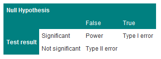
The relationship between Type I and Type II errors is shown in Table 2. One has to imagine a series of cases, in some of which the null hypothesis is true and in some of which it is false. In either situation we carry out a significance test, which sometimes is significant and sometimes not.

The concept of power is only relevant when a study is being planned. After a study has been completed, we wish to make statements not about hypothetical alternative hypotheses but about the data, and the way to do this is with estimates and confidence intervals.

Table 2 Relationship between Type I and Type II errors

Steps to calculating sample size

Usually the significance level is predefined (5% or 1%).

Select the power you want the study to have, usually 80% or 90% (i.e. type II error of 10-20%)

For continuous data, obtain the standard deviation of the outcome measure.

For binary data, obtain the incidence of the outcome in the control group (for a trial) or in the non-exposed group (for a case-control study or cohort study).

Choose an effect size. This is the size of the effect that would be 'clinically' meaningful.

For example, in a clinical trial, the sort of effect that would make it worthwhile changing treatments. In a cohort study, the size of risk that implies a public hazard.

Use sample size tables or a computer program to deduce the required sample size.

Often some negotiation is required to balance the power, effect size and an achievable sample size.

One should always adjust the required sample size upwards to allow for dropouts.

Problems of multiple testing

Imagine carrying out 20 trials of an inert drug against placebo. There is a high chance that at least one will be statistically significant. It is highly likely that this is the one which will be published and the others will languish unreported. This is one aspect of publication bias. The problem of multiple testing happens when:

1. Many outcomes are tested for significance
2. In a trial, one outcome is tested a number of times during the follow up
3. Many similar studies are being carried out at the same time.

The ways to combat this are:

1. To specify clearly in the protocol which are the primary outcomes (few in number) and which are the secondary outcomes.
2. To specify at which time interim analyses are being carried out, and to allow for multiple testing.
3. To do a careful review of all published and also unpublished studies. Of course, the latter, by definition, are harder to find.

A useful technique is the Bonferroni correction. This states that if one is doing n independent tests one should specify the type I error rate as α/n rather than α. Thus, if one has 10 independent outcomes, one should declare a significant result only if the p-value attached to one of them is less than 5%/10, or 0.5%. This test is conservative, i.e. less likely to give a significant result because tests are rarely independent. It is usually used informally, as a rule of thumb, to help decide if something which appears unusual is in fact quite likely to have happened by chance.

Reference

Campbell MJ and Swinscow TDV. Statistics at Square One 11th ed. Wiley-Blackwell: BMJ Books 2009. Chapter 6.

Standard Statistical Distributions (e.g. Normal, Poisson, Binomial) and their uses

Statistics: Distributions

Summary

Normal distribution describes continuous data which have a symmetric distribution, with a characteristic 'bell' shape.

Binomial distribution describes the distribution of binary data from a finite sample. Thus it gives the probability of getting r events out of n trials.

Poisson distribution describes the distribution of binary data from an infinite sample. Thus it gives the probability of getting r events in a population.

The Normal Distribution

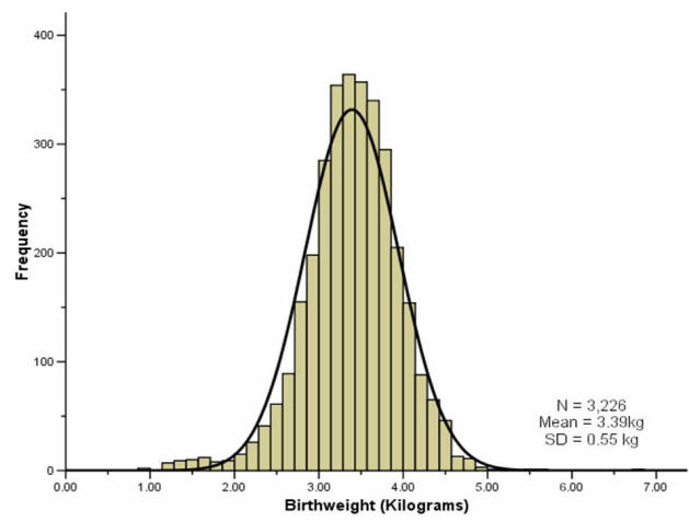
It is often the case with medical data that the histogram of a continuous variable obtained from a single measurement on different subjects will have a characteristic `bell-shaped' distribution known as a Normal distribution. One such example is the histogram of the birth weight (in kilograms) of the 3,226 new born babies shown in Figure 1.

Figure 1 Distribution of birth weight in 3,226 newborn babies (data from O' Cathain et al 2002)

To distinguish the use of the same word in normal range and Normal distribution we have used a lower and upper case convention throughout.

The histogram of the sample data is an estimate of the population distribution of birth weights in new born babies. This population distribution can be estimated by the superimposed smooth `bell-shaped' curve or `Normal' distribution shown. We presume that if we were able to look at the entire population of new born babies then the distribution of birth weight would have exactly the Normal shape. We often infer, from a sample whose histogram has the approximate Normal shape, that the population will have exactly, or as near as makes no practical difference, that Normal shape.

The Normal distribution is completely described by two parameters μ and σ, where μ represents the population mean, or centre of the distribution, and σ the population standard deviation. It is symmetrically distributed around the mean. Populations with small values of the standard deviation σ have a distribution concentrated close to the centre μ; those with large standard deviation have a distribution widely spread along the measurement axis. One mathematical property of the Normal distribution is that exactly 95% of the distribution lies between

$μ - (1.96 x σ) a n d μ + (1.96 x σ)$

Changing the multiplier 1.96 to 2.58, exactly 99% of the Normal distribution lies in the corresponding interval.

In practice the two parameters of the Normal distribution, μ and σ, must be estimated from the sample data. For this purpose a random sample from the population is first taken. The sample mean and the sample standard deviation, $S D (\bar{x}) = S$ , are then calculated. If a sample is taken from such a Normal distribution, and provided the sample is not too small, then approximately 95% of the sample lie within the interval:

\bar{x} - [1.96 \times S D (\bar{x})]

\bar{x} + [1.96 \times S D (\bar{x})]

This is calculated by merely replacing the population parameters μ and σ by the sample estimates and s in the previous expression.

In appropriate circumstances this interval may estimate the reference interval for a particular laboratory test which is then used for diagnostic purposes.

We can use the fact that our sample birth weight data appear Normally distributed to calculate a reference range. We have already mentioned that about 95% of the observations (from a Normal distribution) lie within ±1.96 SDs of the mean. So a reference range for our sample of babies, using the values given in the histogram above, is:

3.39 - [1.96 x 0.55] to 3.39 + [1.96 x 0.55]

2.31kg to 4.47kg

A baby's weight at birth is strongly associated with mortality risk during the first year and, to a lesser degree, with developmental problems in childhood and the risk of various diseases in adulthood. If the data are not Normally distributed then we can base the normal reference range on the observed percentiles of the sample, i.e. 95% of the observed data lie between the 2.5 and 97.5 percentiles. In this example, the percentile-based reference range for our sample was calculated as 2.19kg to 4.43kg.

Most reference ranges are based on samples larger than 3500 people. Over many years, and millions of births, the WHO has come up with a normal birth weight range for new born babies. These ranges represent results than are acceptable in newborn babies and actually cover the middle 80% of the population distribution, i.e. the 10th to 90th centiles. Low birth weight babies are usually defined (by the WHO) as weighing less than 2500g (the 10th centile) regardless of gestational age, and large birth weight babies are defined as weighing above 4000kg (the 90th centile). Hence the normal birth weight range is around 2.5kg to 4kg. For our sample data, the 10th to 90th centile range was similar, 2.75 to 4.03kg.

The Binomial Distribution

If a group of patients is given a new drug for the relief of a particular condition, then the proportion p being successively treated can be regarded as estimating the population treatment success rate .

The sample proportion p is analogous to the sample mean , in that if we score zero for those s patients who fail on treatment, and 1 for those r who succeed, then p=r/n, where n=r+s is the total number of patients treated. Thus p also represents a mean.

Data which can take only a binary (0 or 1) response, such as treatment failure or treatment success, follow the binomial distribution provided the underlying population response rate does not change. The binomial probabilities are calculated from:

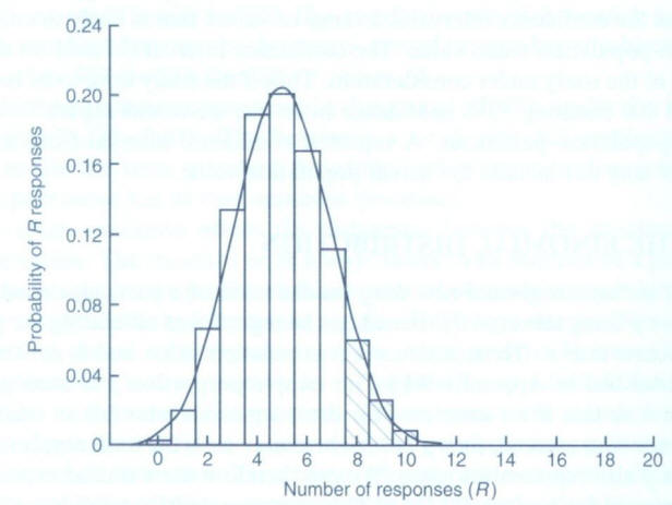
$P (r r e s p o n s e s o u t o f n) = \frac{n!}{r! (n - r)!} π^{r} {(1 - π)}^{n - r}$

…for successive values of R from 0 through to n. In the above, n! is read as “n factorial” and r! as “r factorial”. For r=4, r!=4×3×2×1=24. Both 0! and 1! are taken as equal to 1. The shaded area marked in Figure 2 (below) corresponds to the above expression for the binomial distribution calculated for each of r=8,9,...,20 and then added. This area totals 0.1018. So the probability of eight or more responses out of 20 is 0.1018.

For a fixed sample size n the shape of the binomial distribution depends only on . Suppose n = 20 patients are to be treated, and it is known that on average a quarter, or =0.25, will respond to this particular treatment. The number of responses actually observed can only take integer values between 0 (no responses) and 20 (all respond). The binomial distribution for this case is illustrated in Figure 2.

The distribution is not symmetric, it has a maximum at five responses and the height of the blocks corresponds to the probability of obtaining the particular number of responses from the 20 patients yet to be treated. It should be noted that the expected value for r, the number of successes yet to be observed if we treated n patients, is (nx). The potential variation about this expectation is expressed by the corresponding standard deviation:

$S D (r) = \sqrt{n π (1 - π)}$

Figure 2 also shows the Normal distribution arranged to have μ = n

= 5 and σ = √[n

(1 -

)] = 1.94, superimposed on to a binomial distribution with

= 0.25 and n = 20. The Normal distribution describes fairly precisely the binomial distribution in this case. If n is small, however, or

close to 0 or 1, the disparity between the Normal and binomial distributions with the same mean and standard deviation increases and the Normal distribution can no longer be used to approximate the binomial distribution. In such cases the probabilities generated by the binomial distribution itself must be used.

It is also only in situations in which reasonable agreement exists between the distributions that we would use the confidence interval expression given previously. For technical reasons, the expression given for a confidence interval for a proportion is an approximation. The approximation will usually be quite good provided p is not too close to 0 or 1, situations in which either almost none or nearly all of the patients respond to treatment. The approximation improves with increasing sample size n.

Figure 2: Binomial distribution for n=20 with =0.25 and the Normal approximation

The Poisson Distribution

The Poisson distribution is used to describe discrete quantitative data such as counts in which the population size n is large, the probability of an individual event is small, but the expected number of events, n, is moderate (say five or more). Typical examples are the number of deaths in a town from a particular disease per day, or the number of admissions to a particular hospital.

Example

Wight et al (2004) looked at the variation in cadaveric heart beating organ donor rates in the UK. They found that there were 1330 organ donors, aged 15-69, across the UK for the two years 1999 and 2000 combined. Heart-beating donors are patients who are seriously ill in an intensive care unit (ICU) and are placed on a ventilator.

Now it is clear that the distribution of the number of donors takes integer values only, thus the distribution is similar in this respect to the binomial. However, there is no theoretical limit to the number of organ donors that could happen on a particular day. Here the population is the UK population aged 15-69, over two years, which is over 82 million person years, so in this case each member can be thought to have a very small probability of actually suffering an event, in this case being admitted to a hospital ICU and placed on a ventilator with a life threatening condition.

The mean number of organ donors per day over the two year period is calculated as:

$r = \frac{1330}{(365 + 365)} = \frac{1330}{730} = 1.82$ organ donations per day

It should be noted that the expression for the mean is similar to that for , except here multiple data values are common; and so instead of writing each as a distinct figure in the numerator they are first grouped and counted. For data arising from a Poisson distribution the standard error, that is the standard deviation of r, is estimated by SE(r) = √(r/n), where n is the total number of days (or an alternative time unit). Provided the organ donation rate is not too low, a 95% confidence interval for the underlying (true) organ donation rate λ can be calculated in the usual way:

$r - [1.96 \times S E (r)] t o r + [1.96 \times S E (r)]$

In the above example r=1.82, SE(r)=√(1.82/730)=0.05, and therefore the 95% confidence interval for λ is 1.72 to 1.92 organ donations per day. Exact confidence intervals can be calculated as described by Altman et al. (2000).

The Poisson probabilities are calculated from:

$P (r r e s p o n s e s) = \frac{λ^{r}}{r!} e^{- λ}$

…for successive values of r from 0 to infinity. Here e is the exponential constant 2.7182…, and λ is the population rate which is estimated by r in the example above.

Example

Suppose that before the study of Wight et al. (2004) was conducted it was expected that the number of organ donations per day was approximately two. Then assuming λ = 2, we would anticipate the probability of 0 organ donations in a given day to be (20/0!)e-2 =e-2 = 0.135. (Remember that 20 and 0! are both equal to 1.) The probability of one organ donation would be (21/1!)e-2 = 2(e-2) = 0.271. Similarly the probability of two organ donations per day is (22/2!)e-2= 2(e-2) = 0.271; and so on to give for three donations 0.180, four donations 0.090, five donations 0.036, six donations 0.012, etc. If the study is then to be conducted over 2 years (730 days), each of these probabilities is multiplied by 730 to give the expected number of days during which 0, 1, 2, 3, etc. donations will occur. These expectations are 98.8, 197.6, 197.6, 131.7, 26.3, 8.8 days. A comparison can then be made between what is expected and what is actually observed.

Other Distributions

A brief description of some other distributions are given for completeness.

t-distribution

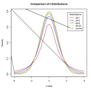
Student’s t-distribution is a continuous probability distribution with a similar shape to the Normal distribution but with wider tails. t-distributions are used to describe samples which have been drawn from a population, and the exact shape of the distribution varies with the sample size. The smaller the sample size, the more spread out the tails, and the larger the sample size, the closer the t-distribution is to the Normal distribution (Figure 3). Whilst in general the Normal distribution is used as an approximation when estimating means of samples from a Normally-distribution population, when the same size is small (say n<30), the t-distribution should be used in preference.

Figure 3. The t-distribution for various sample sizes. As the sample size increases, the t-distribution more closely approximates the Normal.

Chi-squared distribution

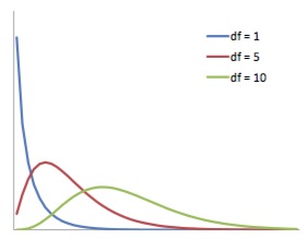
The chi-squared distribution is continuous probability distribution whose shape is defined by the number of degrees of freedom. It is a right-skew distribution, but as the number of degrees of freedom increases it approximates the Normal distribution (Figure 4). The chi-squared distribution is important for its use in chi-squared tests. These are often used to test deviations between observed and expected frequencies, or to determine the independence between categorical variables. When conducting a chi-squared test, the probability values derived from chi-squared distributions can be looked up in a statistical table.

Figure 4. The chi-squared distribution for various degrees of freedom. The distribution becomes less right-skew as the number of degrees of freedom increases.

References

Statistics Notes BMJ http://bmj.bmjjournals.com/cgi/content/full/329/7458/168
Campbell MJ, Machin D and Walters SJ. Medical Statistics: a Commonsense Approach 4th ed. Chichester: Wiley-Blackwell 2007 Chapter 4
Campbell MJ and Swinscow TDV Statistics at Square One. 11th ed Oxford; BMJ Books Blackwell Publishing 2009 Chapter 9

Tace News and Tutorials call 07062211611 for WAEC, JAMB Tutorials Web design, Social Media Marketng

Search This Blog

Probability bases to advanced

Health Knowledge

Elementary Probability Theory

Statistics: Elementary Probability Theory

Regression and correlation

Regression and correlation

Statistics: Correlation and Regression

Sampling Distributions

Sampling Distributions

Statistics: Significance testing, Type I and Type II errors

Standard Statistical Distributions (e.g. Normal, Poisson, Binomial) and their uses

Standard Statistical Distributions (e.g. Normal, Poisson, Binomial) and their uses

Statistics: Distributions

Our most popular content

Recently updated content